Introducing PeaCoq
What is PeaCoq?
Over the past year, I have developed a Coq frontend called PeaCoq (not to be mistaken with Yves Bertot’s Pcoq). If you wish to play with it before or while reading this article, I made an online version available here. Note that it will reset after 15 minutes of inactivity, and that it might go down any time!
There have been several attempts at improving user interfaces for proof assistants, so I will describe here some of PeaCoq’s features. I built PeaCoq with the goal of helping both novice and more advanced users. I chose to build it as a web-based text editor, so that it was easy to have people try it. The client-server architecture means PeaCoq users only need a web browser to interact with a Coq session hosted on the server. Unfortunately, this means PeaCoq does not run in your favorite text editor.
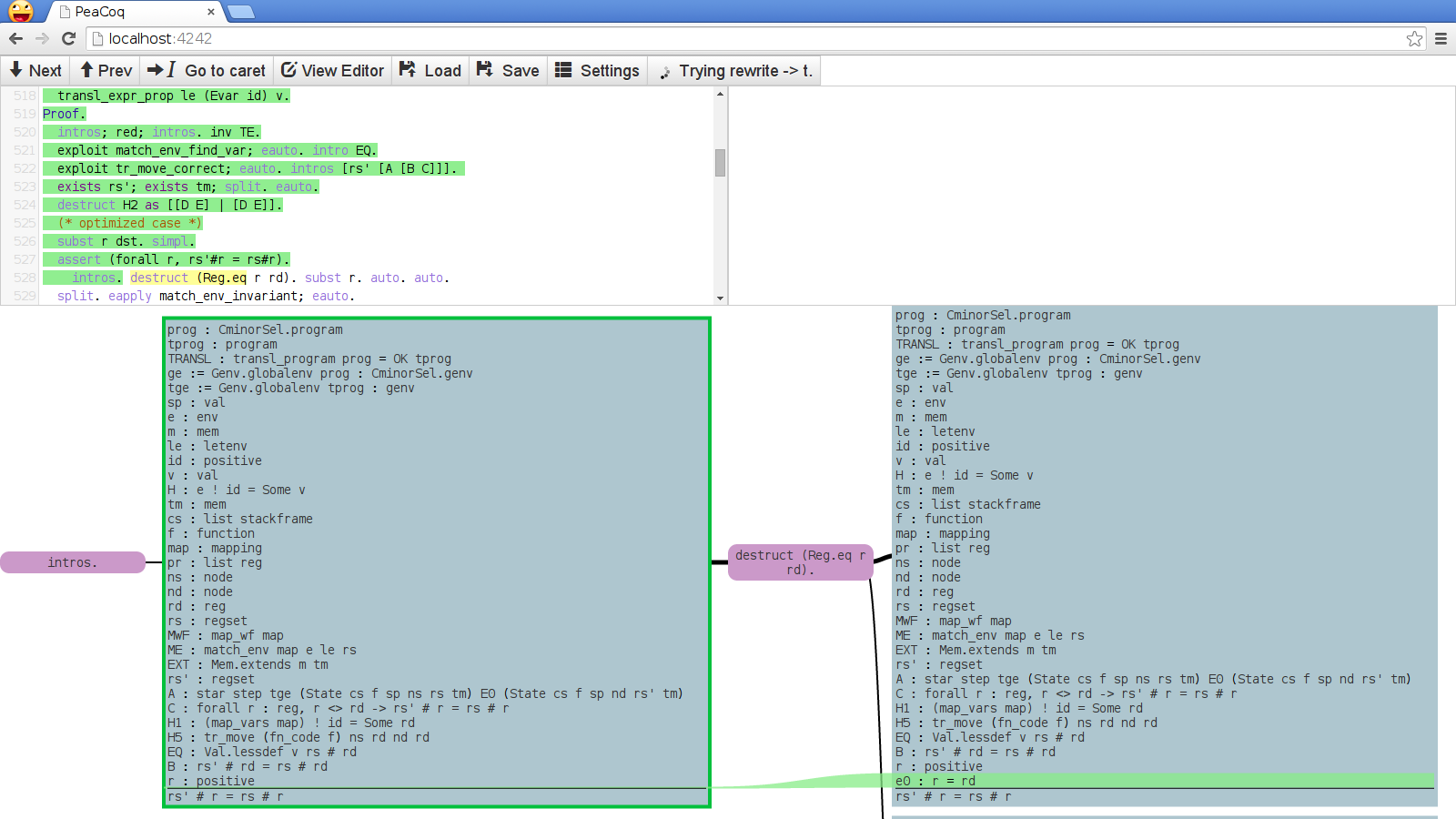
The main feature of PeaCoq is its tree mode. Whenever you enter a proof, the interface splits into this view:
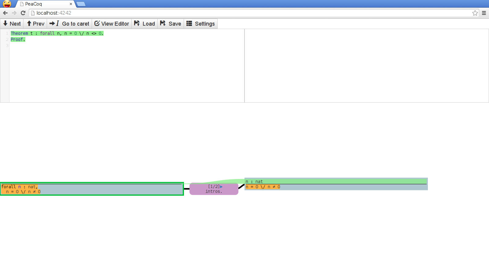
The top part of the screen has your editor on the left, and a buffer for errors on the right. The bottom part shows your current proof context in the leftmost rectangle, a tactic in the purple node, and the resulting proof context in the right rectangle.
In the next sections, I will discuss two features of PeaCoq: the automated trial of tactics in the background, and the highlighting of the differences between proof contexts.
Automatically trying tactics
Like most programming languages, learning Coq requires making yourself familiar with a vernacular of syntactic elements and their proper grammar. In fact, Coq has three languages whose interaction is crucial to achieve anything:
Vernacular, the language used to introduce constructs and change meta-level properties
Gallina, the language used to define computational behaviors
Ltac, the language used to interact with proof contexts.
Learning these three languages can be overwhelming. To bridge some of this “gap
of execution”, PeaCoq can try tactics in the background, and display the results
to the user. We only show the result of tactics that succeed and actually modify
the context. This way, we avoid displaying tactics that may succeed yet do
nothing, like firstorder.
The first challenge here is to pick a suitable set of tactics to try. Some tactics are benign to try all the time, while some tactics can take a very long time to succeed or fail. So far, we have only used a set of curated tactics, and try them in order of their expected complexity.
Now, most tactics have a plethora of arguments and variants that are sometimes useful, sometimes necessary to use in order to make progress. For instance, introduction tactics let you specify names or even deconstruction patterns. Rewrite tactics let you specify which occurence of the unified pattern to actually perform the rewrite on. Existential tactics need you to provide an existential witness. It is unclear how to cater for all of these. By default, PeaCoq will only try very simple things: it will not name introduced variables, it will try all rewrites in all directions for all names in local context, over all hypotheses and the goal. This quickly grows big, though in practice many of these tactics immediately fail.
Another problem is in displaying the succesful tactics. There usually are many succesful tactics, with often redundant results. In order to display sometimes dozens of goals, PeaCoq groups them in a two-dimensional fashion. So far, we group tactics by their purpose (introduction tactics, rewrite tactics, solvers, etc.).
Highlighting differences between proof contexts
Here the problem seems simple. Assuming you have parsed the proof context before and after running a tactic, I would like to identify a set of differences. These differences can be:
- the appearance or disappearance of a hypothesis
- the reordering of a hypothesis
- a set of structural changes within a hypothesis or the goal
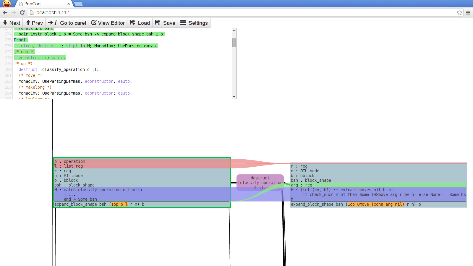
where the last two may overlap. Here is an example of the visualization of such a changeset:
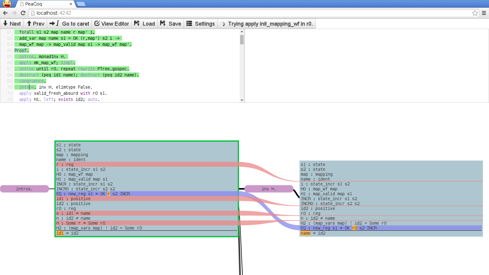
The red, shrinking streams indicate hypotheses that disappear. The blue stream indicates the repositioning of a hypothesis. The orange patches indicate changes in the structure of a term.
Computing the streams is not too difficult. The interesting part is in computing differences within terms.
There has been some research on computing differences between abstract syntax trees, mostly in order to highlight changes between versions of software. They are somewhat too complicated for our intent as they often also compute code movement.
The naïve approach here is to compute similarity top-down and highlight subnodes of the AST that differ. This is a good first approximation, but it may give some non-intuitive results. For instance, consider the simplification step from:
1
| |
to
1
| |
This algorithm would see that the top-level node is an application node on both
sides, and would recursively highlight concat (cons n l) as being different
from cons n, and nil as being different from (concat l nil) (remember,
function application is left-associative). This is often confusing because the
entire term looks different, and the fact that the application node is still an
application node is somewhat insignificant. In these situations we want to lift
the difference to the entire application.
This still leaves an issue. Consider the following:
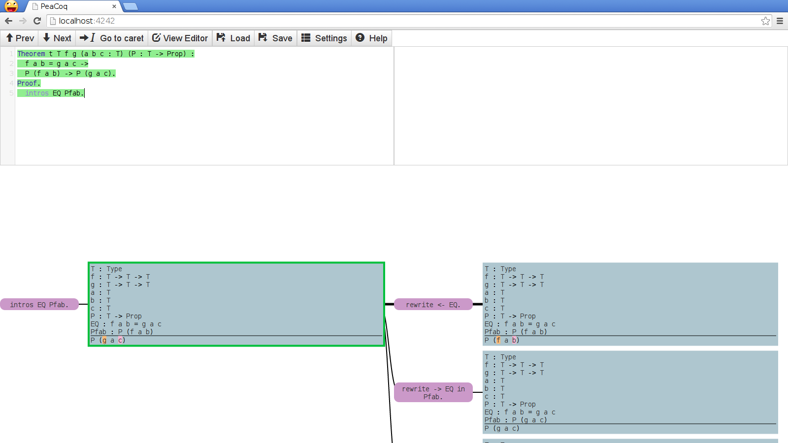
Even though the algorithm is precise in identifying that only the function being
applied and its second argument have changed, this diff is somewhat misleading
as to the semantics of rewrite. It might be better to highlight the entire
expression f a b as modified. I am currently toying with this idea, thinking
of bubbling differences whenever a nested application has both a modified
functional term and a modified argument. The bubbling could propagate all the
way to the last modified argument. Of course, it would over-approximate cases
where the tactic actually intended to modify only these two precise locations. I
don’t know if this is often the case.
A last concern is the detection of generalization or instantiation of quantifiers. The current algorithm flags the entire term as different whenever the top-most node in the AST differs, which is unfortunate for quantifier instantiation when the resulting subgoal is a subterm of the original subgoal or vice-versa. Ideally, I would find the matching subtree, and somehow indicate visually that only the quantifier has disappeared.
Evaluating PeaCoq for novices
I have been trying to evaluate PeaCoq since January. During the winter quarter, Zachary Tatlock taught the graduate programming languages class at University of Washington using PeaCoq as the in-class editor and as an option for students.
Students were overall positive about PeaCoq, even though the version they use was very unstable and undergoing development while they were working with it. Some students chose not to use PeaCoq, either because they already had their own ProofGeneral setup, or because they had a bad experience with PeaCoq. At that time, the editor was primitive, the proof tree feature was very brittle, and it was impossible to switch in and out of the proof tree mode on the fly. Many of these problems are now solved!
While this was overall a positive experience, I felt I needed more conclusive evidence of the help provided by PeaCoq for beginners, so I set up an A-B study. I recruited 20 graduate students, randomly assigned pairs of them into one of two groups, and had them work through a one-hour lecture followed by a one-hour exercise session. Group A was to perform the exercises in a ProofGeneral setting, while group B used PeaCoq’s trees. Here is the averaged data per exercise.
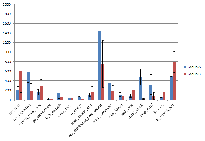
As you can see, the data is fairly inconclusive, partly because of flaws of the
study setup. Hours before the study started, I removed a lemma that made
rev_distributes_over_concat easier to prove. Students in group A were
extremely stuck, though two pairs found a solution that involved a sequence of
five rewrites. Four out of five pairs in group B found that solution too. After
a long period of time, we unlocked everyone.
Ignoring this exercise, we can notice a few things. In the first exercise, the control group was much faster than group B! It turns out, some groups got lost looking at all the options PeaCoq proposed, rather than trying things boldly. On the other hand, the control group had to try things without any preview, and therefore tried to apply the same technique as in the in-class exercises, which was exactly the right way to go.
Another issue that came up was the abundance of spurious options offered by PeaCoq. For instance, we introduced lemmas like:
1
| |
or
1
| |
Therefore, upon mining for rewrite possibilities, PeaCoq would offer many
spurious rewrites, like rewrite <- concat_nil_right., every time a list was in
context. This tactic replaces l with concat l nil, which, while correct, is
most often not something you would like (unless you wanted to put the goal in
this shape to apply some lemma).
It would be nice to filter such options, either by indicating to PeaCoq that some rewrites are only helpful in one direction, or by having a smarter metric for complexity.
map'_unroll was very PeaCoq-friendly in that it was a goal that held by
reflexivity while not looking reflexive, and would not simplify by
simpl. PeaCoq users were immediately presented with a reflexivity. node,
while most of the control group got stuck and asked me what to do.
The latter exercises were only reached by a few pairs of the control group within the allocated time (thus the null standard deviation).
Overall, while it seemed PeaCoq was very helpful in some places, there were many confounding factors and places were the options offered by PeaCoq were more overwhelming than helpful for novices.
I am working on alleviating some of these pitfalls, and hopefully another study will highlight the benefits of PeaCoq…
Other challenges and features
Parsing Coq terms: Up to version 8.4, the protocol used in communicating with a coqtop process was fairly terrible. In particular, terms were exchanged as strings, which made the kind of techniques used to display term differences challenging. My current solution is equally unsatisfactory: I wrote a small parser for Coq’s syntax. It does not handle everything, in particular notations, and so fails to parse many terms. Upon failure, the diff feature takes the conservative approach of string comparison. Coq 8.5 seems to finally output ASTs, so hopefully PeaCoq could leverage this to avoid recomputing all this information!
Generate robust proofs: ideally, I would like editor support to make my proofs more robust. One pitfall when using theorem provers is how boring it is to introduce names, but how practical they are to use to quickly refer to something. This makes for proofs scripts were names are automatically introduced, and are therefore very brittle to small changes. It would be nice if the editor could prevent one from using automatically-introduced names, or retroactively edit the proof to introduce the name “auto-manually” once it is used, by keeping track of where it appeared and when it is used!
Reducing context clutter: consider the following screenshot, taken from somewhere within a proof in CompCert.
So many lines! In my experience, there is little value in having all those lines most of the time. In particular, I am often interested in hypotheses that have indexed types, and not so much in the others, that are just “data”. Here is what I envision instead for PeaCoq:
All the variables in context but whose type is of lesser interest have been removed. You should be able to access them somehow (maybe by hovering your mouse wherever they appear? maybe by some keyboard shortcut query? maybe they should still be visible in some folded pane?), but I don’t want them in my way most of the time. Of course there would be tricky interactions with the diff feature.
I would also like to be able to make hypotheses as “hidden” without necessarily hiding them in the proof script.
- Manipulating the structure of terms: Now consider this context.

This long unfolded term takes the entire screen space. I rarely need to see this unfolded version, and PeaCoq knows the structure of the term and has built a DOM object with the proper structure, I should be able to have this long term be folded, and only unfolded if I want to. I have not implemented this yet, but I would like it to look something like:
(Oops, there is a slight but in the stream algorithm!)
- Supporting Coq’s evolution: In general, it would be nice to stay up-to-date, in particular to support Coq’s new background processing mechanism. Now this would make for some non backwards-compatible changes, so I’d rather wait until the community switches to 8.5.
That’s all folks!
If you want to see or talk about PeaCoq, I will be attending PLDI in Portland
next week! You can also find me as Ptival on #coq or email me!
The project lives on GitHub. Please report bugs or suggestions for enhancements! :)